Neural Network For Fashion Mnist
A classic dataset for evaluation of a computer vision network is the Fashion MNIST Dataset. This dataset consists of 70,000 28X28 pixels of different clothing items split into a 60,000 unit training set and a 10,000 unit test set. There are equal numbers of all clothing items within these items. It looks like this:
![]()
Benchmark Accuracy
The creators of this dataset have supplied accuracy scores for each of the machine learning models built into the popular sci-kit learn package. We can see that the competitive models perform at or around the 85% to 90% accuracy mark. This provides a good benchmark for evaluating our neural net.
Building the Network
Our network is going to consist of 3 parts:
- A Flatten layer that will convert the images into an array that our model can understand.
- 2 hidden layers that will process this array,
- An output layer that will return a guess at the correct class for this item.
The initial layer can be constructed using the Flatten layer of the tensorflow.keras package:
net = Sequential()
net.add(Flatten(input_shape=(28, 28)))
Note that we pass the input_shape argument with the size of our image.
We then add a simple 2 layer processing step using the Dense layer from the tensorflow.keras package:
net.add(Dense(30, activation="relu"))
net.add(Dense(20, activation="tanh"))
Then we add the output layer. As there are 10 possible options in our data set, it must be 10 nodes in size.
net.add(Dense(10, activation="softmax"))
Finally, we can compile and fit the model to the data.
net.compile(loss="sparse_categorical_crossentropy", metrics=["accuracy","mse"])
net.fit(x_train, y_train, epochs=10, batch_size=25, callbacks=[tensorboard_callback])
To run this with the Fashion MNIST data we can use the below code:
import os
import datetime
import tensorflow as tf
import pandas as pd
import numpy as np
import matplotlib.pyplot as plt
import seaborn as sns
from tensorflow.keras.models import Sequential
from tensorflow.keras.layers import Dense, Flatten
from sklearn.metrics import confusion_matrix, plot_confusion_matrix

logdir = os.path.join("logs", datetime.datetime.now().strftime("%Y%m%d-%H%M%S"))
tensorboard_callback = tf.keras.callbacks.TensorBoard(logdir, histogram_freq=1)

(x_train, y_train), (x_test, y_test) = tf.keras.datasets.fashion_mnist.load_data()

x_train = x_train.astype(np.float32) / 255.0
x_test  = x_test.astype(np.float32) / 255.0

LABELS = \
  [ "T-shirt/top"
  , "Trouser"
  , "Pullover"
  , "Dress"
  , "Coat"
  , "Sandal"
  , "Shirt"
  , "Sneaker"
  , "Bag"
  , "Ankle boot"
  ]

net = Sequential()
net.add(Flatten(input_shape=(28, 28)))
net.add(Dense(30, activation="relu"))
net.add(Dense(20, activation="tanh"))
net.add(Dense(10, activation="softmax"))
net.compile(loss="sparse_categorical_crossentropy", metrics=["accuracy","mse"])
net.fit(x_train, y_train, epochs=10, batch_size=25, callbacks=[tensorboard_callback])
This should output something like:
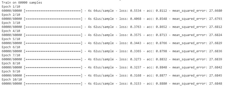
Considering the benchmarks, 88% accuarcy is not bad!
Evaluating the Model
Let’s first evaluate the model’s predictions by eye. This is a simple function to print an example and the model’s guess.
def ShowPrediction(test):
  plt.figure(figsize=(2,2))
  plt.imshow(x_test[test], cmap="gray")
  plt.xlabel(LABELS[net.predict_classes(x_test[test:test+1])[0]])
  plt.show()
If we try this function on x_test[666] we should see:
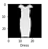
This would seem correct. After trying a few examples, let’s move on to:
score = net.evaluate(x_test, y_test)[1]
print(f"Model is {round(score*100,2)}% accurate")
Which returns:
Model is 85.55% accurate
Slightly worse than our training result.
Confusion Matrix
We can also visualise these results as a confusion matrix to review which classes are frequently confused:
plt.figure(figsize=(10,10))
sns.set(style="whitegrid", context="notebook")

y_guess = [LABELS[x] for x in net.predict_classes(x_test)]
y_true = [LABELS[x] for x in y_test]

cm = confusion_matrix(y_true, y_guess, normalize=None)
ax = sns.heatmap(cm, annot=True, cmap="Blues", fmt="d", xticklabels=LABELS, yticklabels=LABELS, cbar=False)
Which outputs:
.png)
This shows us that the most frequently confused classes are “Bag” and “Shirt”
I will revisit this model in a future post