Improving Fashion Mnist With Convolutions
This is a follow-up post to the initial model presented here
Starting from our baseline fully connected neural net code.
import os
import datetime
import tensorflow as tf
import numpy as np
from tensorflow.keras.models import Sequential
from tensorflow.keras.layers import Dense, Flatten

(x_train, y_train), (x_test, y_test) = tf.keras.datasets.fashion_mnist.load_data()

x_train = x_train.astype(np.float32) / 255.0
x_test  = x_test.astype(np.float32) / 255.0

LABELS = \
  [ "T-shirt/top"
  , "Trouser"
  , "Pullover"
  , "Dress"
  , "Coat"
  , "Sandal"
  , "Shirt"
  , "Sneaker"
  , "Bag"
  , "Ankle boot"
  ]

net = Sequential()

net.add(Flatten(input_shape=(28, 28)))
net.add(Dense(30, activation="tanh"))
net.add(Dense(20, activation="tanh"))
net.add(Dense(10, activation="softmax"))
net.compile(loss="sparse_categorical_crossentropy", metrics=["accuracy","mse"])
net.fit(x_train, y_train, epochs=10, batch_size=25)

score = net.evaluate(x_test, y_test)[1]
print(f"Model is {round(score*100,2)}% accurate")
We can recall that this code scored 85.55% on the test set of our Fashion MNIST data set. Which is a fairly good result for such a simple network.
To attempt to improve this score we can include some alterations to the input image in order for our model to better understand the inputs.
Convolutions
One operation that we can try is applying convolutions to the image. A convolution is a far more efficient way of flattening the image input into a format that the NN can understand.
To do this the convolution cycles through smaller slices of the image and applys an aggregation function to detwermine the most important items to retain.
The above image indicates a convolution with the kernel size of 3X3 cycling through a 4X4 layer.
The above gif demonstrates the max ppoling of values in a 9-square grid down to a single value.
Incorporating Convolutions Into Our Model
We can incorporate this operation into our model through the use of the Tensorflow Conv2D layer ahead of our flatten layer.
The arguments provided here are the filter (16) and the kernel size (3 by 3).
net.add(Conv2D(filters=16, kernel_size=(3, 3), activation="tanh", padding="same"))
We can then provide the MaxPool2D layer to aggregate these values.
net.add(MaxPool2D(pool_size=(2, 2), strides=None, padding="same"))
Our full model is as below:
net = Sequential()
net.add(Conv2D(filters=16, kernel_size=(3, 3), activation="tanh", padding="same"))
net.add(MaxPool2D(pool_size=(2, 2), strides=None, padding="same"))
net.add(Flatten(input_shape=(28, 28)))
net.add(Dense(30, activation="tanh"))
net.add(Dense(20, activation="tanh"))
net.add(Dense(10, activation="softmax"))
net.compile(loss="sparse_categorical_crossentropy", metrics=["accuracy","mse"])
net.fit(x_train, y_train, epochs=10, batch_size=100, callbacks=callbacks)
score = net.evaluate(x_test, y_test)[1]
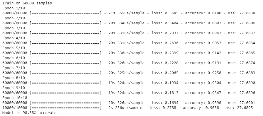
print(f"Model is {round(score*100,2)}% accurate")
Adding these 2 layers to the model increase the accuracy to 90.38%